Forecasting

Time-series forecasting on the sensor data using SARIMAX (Seasonal AutoRegressive Integrated Moving Average with eXogenous factors) from statsmodels.

The full notebook is in the air-quality-data-analysis repository (notebooks/prediction.ipynb).

Warning

The forecasting results here are not great. This was an early attempt at time-series forecasting as part of a university project and the approach has several issues outlined below. Documenting what went wrong is part of the learning process.

Approach

1. Load ~30 days of sensor data from InfluxDB (or from a cached CSV)
2. Resample to 1-hour intervals and interpolate missing values
3. Split into 80% train / 20% test
4. Fit SARIMAX models for temperature, pressure, and humidity
5. Generate predictions on the test set and compare against observed values

Data preparation

The raw data comes in at ~1-second intervals. For forecasting, it's resampled to hourly means and interpolated:

df = sensor.copy().resample("1h").mean()
df = df.apply(lambda x: x.interpolate(method="time"))

train_size = int(len(df) * 0.8)
train, test = df[:train_size], df[train_size:]

This gives about 341 training samples and 85 test samples (in hours).

ACF and PACF analysis

Autocorrelation (ACF) and partial autocorrelation (PACF) plots were used to determine the order parameters for each SARIMAX model.

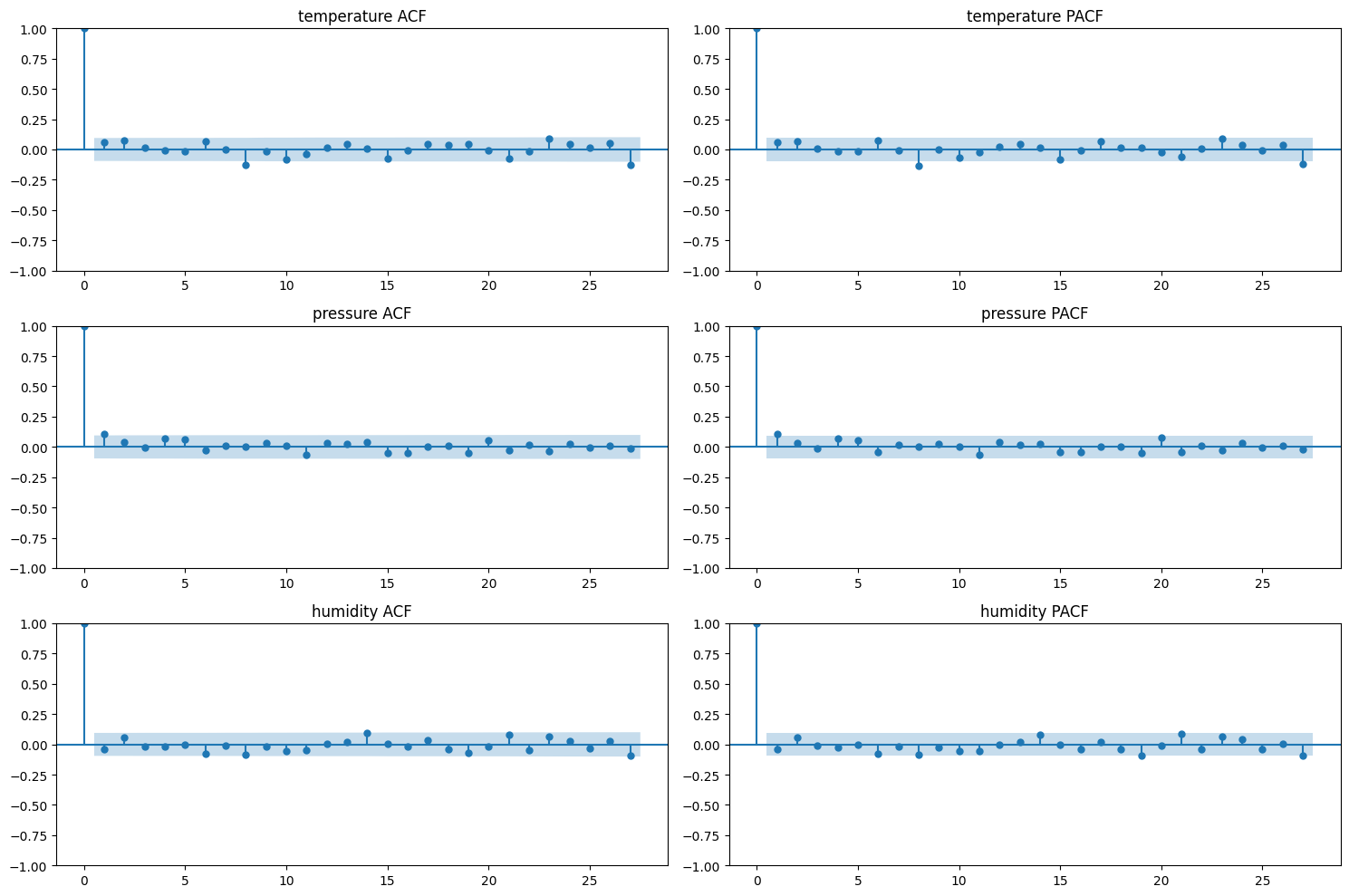
Here's where the first problem shows up. All three parameters (temperature, pressure, humidity) have almost no significant autocorrelation beyond lag 0. The ACF drops to near-zero immediately and stays within the confidence bands. This means the hourly-resampled data behaves almost like white noise - each hour's reading is barely correlated with the previous one.

This makes sense for a controlled indoor environment - the hourly averages don't move much from one hour to the next, and when they do move, it's driven by external factors (weather, human activity) that aren't captured in the univariate time series.

In retrospect, these ACF/PACF plots were a signal that SARIMAX was not the right tool for this data. The lack of autocorrelation means there isn't much temporal structure for the model to learn from.

Model parameters

Despite the flat ACF/PACF, the models were fitted with fairly high order parameters:

Parameter	Order (p,d,q)	Seasonal order (P,D,Q,s)
Temperature	(8, 0, 8)	(2, 0, 0, 24)
Pressure	(11, 0, 11)	(2, 0, 0, 24)
Humidity	(14, 0, 27)	(2, 0, 0, 24)

These high orders were likely a mistake - the ACF/PACF plots don't support orders this high. The seasonal period s=24 (daily cycle in hourly data) is reasonable in theory, but the data doesn't show strong daily seasonality because the sensor is indoors.

The humidity model in particular has an AR order of 14 and MA order of 27 - that's a lot of parameters for 341 training samples. This almost certainly leads to overfitting.

Results

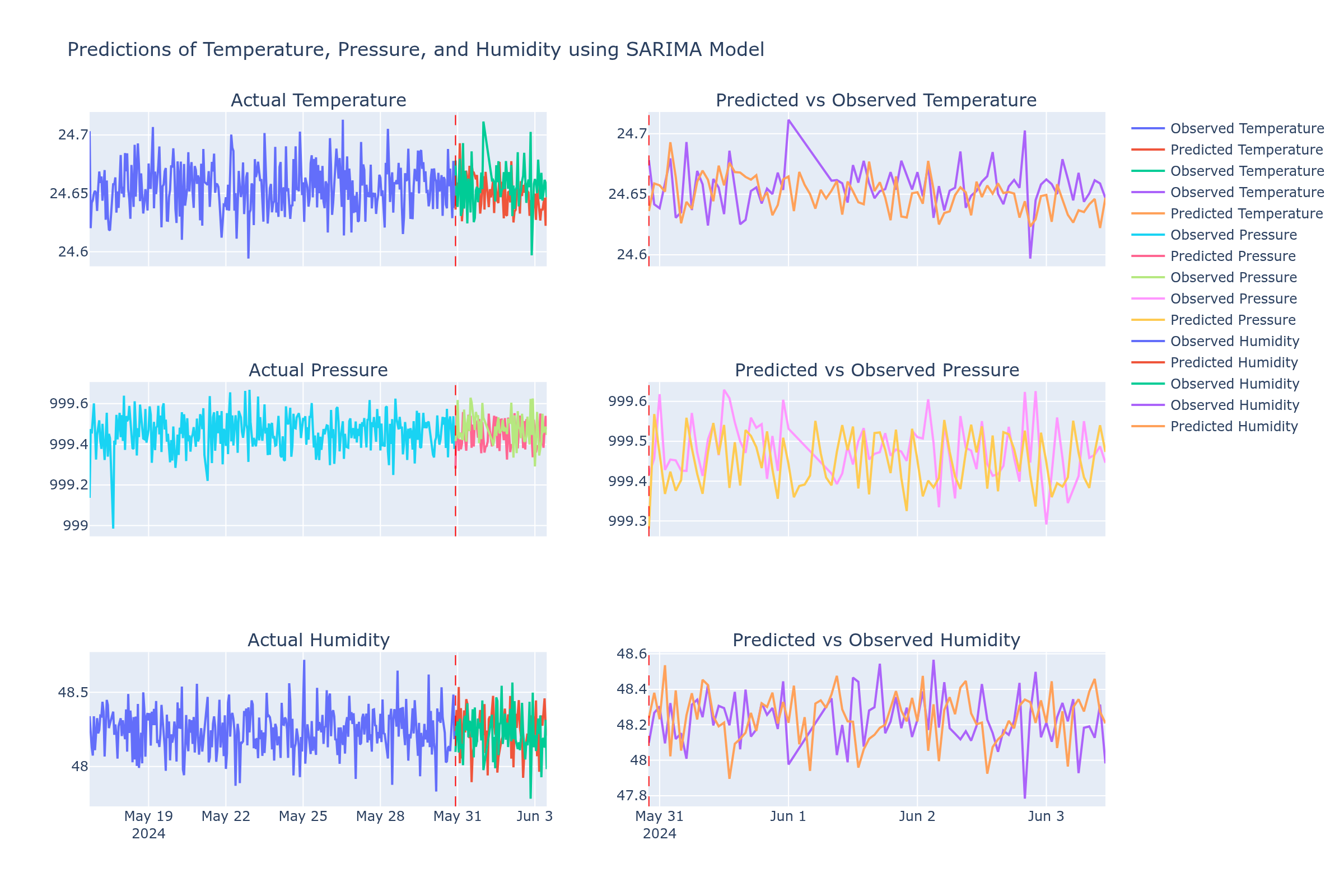
The left column shows the full observed data with predictions overlaid (red dashed line marks the train/test split). The right column zooms into the test period.

Temperature predictions

The temperature prediction (top row) roughly follows the observed values - it captures the general range (24.5-24.7C) but misses the actual fluctuations. It mostly oscillates around the mean, which is not much better than just predicting the average temperature.

Pressure predictions

Pressure (middle row) is the most interesting case. The predictions track the general direction of pressure changes in some places, but the amplitude is off - the model predicts larger swings than what actually happens. Pressure has the most natural variation in this dataset (driven by weather), which gives the model something to work with, but the short training period isn't enough to learn weather patterns well.

Humidity predictions

Humidity (bottom row) is where the model clearly fails. The predictions diverge significantly from observed values, swinging wildly between ~47.8 and 49.5 while the actual humidity is more stable. This is the model with 14 AR and 27 MA terms overfitting to noise in the training data and then producing unstable predictions on new data.

What went wrong

Looking back at this honestly:

1. Wrong interpretation of ACF/PACF - the plots showed no significant autocorrelation, which should have been a sign to try a different approach, not to increase model order. High model orders were chosen hoping to capture something that wasn't really there.

2. Too little data - ~14 days (341 hourly samples) is not enough for SARIMAX with a 24-hour seasonal period. The model needs multiple full cycles of the seasonal pattern to learn it.

3. Overfitting - especially the humidity model with 41 total AR+MA parameters fitted on 341 samples. The model memorized training noise instead of learning actual patterns.

4. Indoor environment - SARIMAX works best on data with clear trends and seasonal patterns (e.g., outdoor temperature over months). Indoor sensor data in a climate-controlled room is too stable for time-series forecasting to add much value.

5. No stationarity testing - the notebook doesn't run an ADF (Augmented Dickey-Fuller) test or other stationarity check before fitting. The d=0 (no differencing) in all models assumes the data is already stationary, which may not be accurate for pressure.

What would actually work better

• More data - collect for months, not days, to capture actual seasonal patterns
• Simpler models - given the near-white-noise ACF, a simple moving average or exponential smoothing would perform about the same with far less complexity
• Multivariate approach - use external data (outdoor weather forecasts) as exogenous variables in SARIMAX, since indoor conditions are largely driven by outdoor weather
• Different algorithms - Prophet, LSTM, or even a simple linear regression against outdoor weather data would likely outperform univariate SARIMAX on this dataset
• Better validation - use cross-validation instead of a single train/test split, and measure actual error metrics (RMSE, MAE) rather than just eyeballing the plots